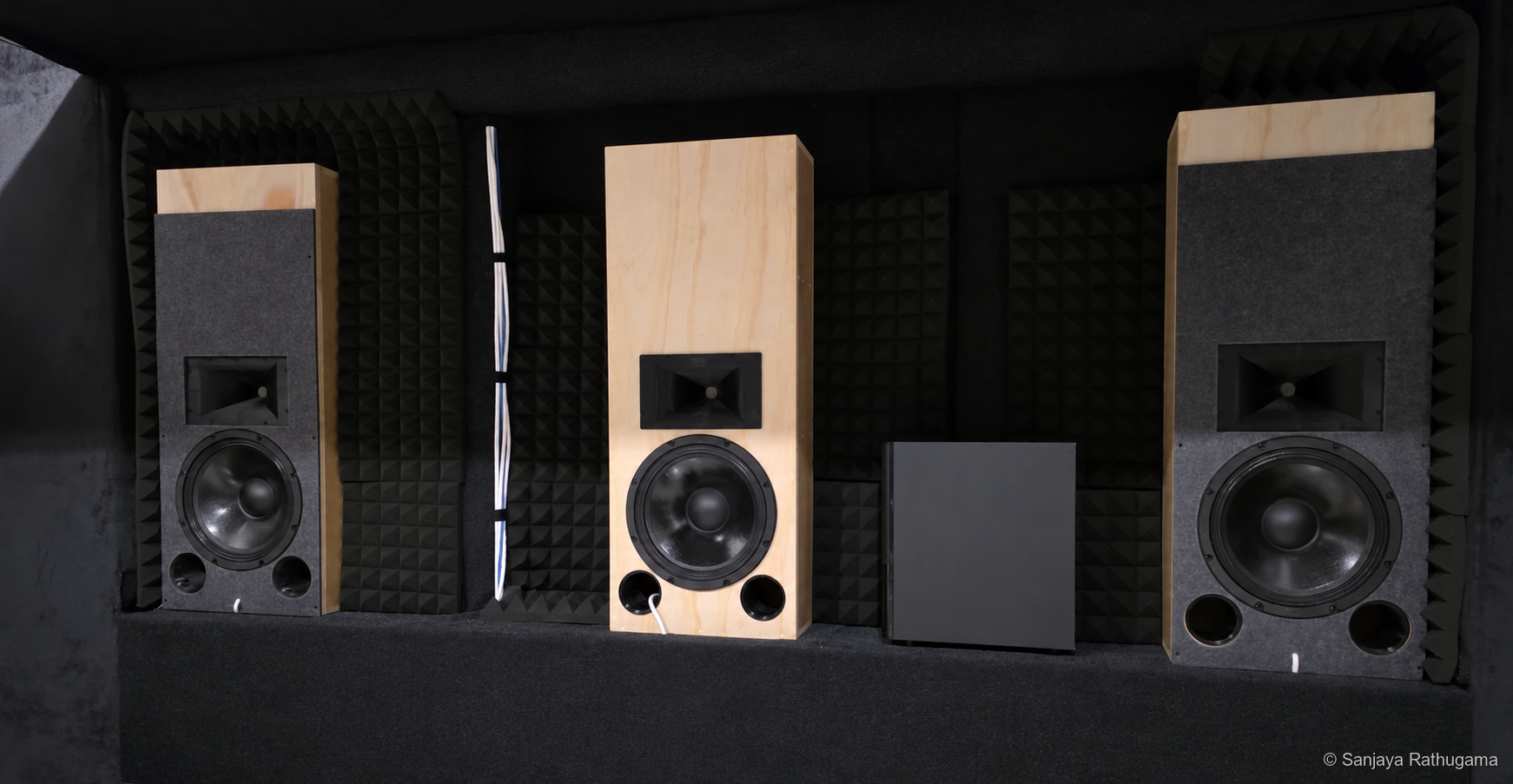
The projector had already changed how I used the room. Next came the front stage: three matching speakers for the left, centre and right channels, with enough output margin for demanding soundtracks and dimensions that worked around the larger picture.
Since I was taking on both the design and the build, I wanted to go a bit wild with it. My ambition was to build a front stage that could compete with very expensive, high-end home theatre speakers: clear dialogue, convincing dynamics and enough headroom to make demanding scenes feel effortless. Doing it myself gave me the freedom to choose the drivers, design the horns and shape the enclosures around exactly what I needed.
As an engineer, part of the attraction was seeing how much performance I could achieve for the money. I wanted to build something exceptional at a low cost, putting my own design work, fabrication and testing into the project to make the budget go further. Choosing where to spend mattered: capable drivers, a well-integrated crossover and an enclosure that worked in the room all had to earn their place. The ambition was high-end performance at a fraction of the price of an expensive commercial system. The cost of my own evenings and weekends was, of course, conveniently left out of that calculation.
I also wanted the experience to feel like a cinema, with sound and picture belonging together. Putting all three front speakers behind the screen was important to that idea. In particular, I wanted dialogue to feel anchored to the people and action on screen, with the centre channel behind the image and the left and right channels supporting the soundstage across it. A voice drawing attention to a box above or below the picture would take something away from that illusion.
That called for an acoustically transparent projection screen, allowing sound from the speakers to pass through the image surface. It also made the screen material and the spacing in front of the speakers part of the acoustic design. The aim was a front stage that felt integrated with the picture, while preserving the placement and aiming the speakers needed.
The front wall was a framed structure at the screen end of the room, housing the three speakers and the acoustic treatment around them. It brought the front stage together while giving me a way to use the existing window recess for the enclosures.
There was one awkward detail. The room is only about four metres deep. A deep enclosure behind a new front wall would take space away from the seats, so I planned to use the window recess and sill area to push the speakers back. That put the cabinet depth at around 200 mm before I had settled the rest of the design.
I had already built an 8-inch horn-loaded prototype to learn about compression drivers, horns and crossover development. It made the unfamiliar parts manageable, but the prototype woofer's available displacement left me wanting more output margin for the front stage. This time I wanted to take those lessons into three larger speakers, designed around the room and the system they would actually be used with. I also moved from the prototype's BIANCO-44CD-K compression driver to the ROSSO-44CD-PK, making the final driver combination another part of the design to measure and develop.
Designed for the complete system
These LCRs were designed to work with large subwoofers, an AVR and an Emotiva XPA-7 Gen3. The AVR handles decoding, levels, delays and bass management; three Emotiva channels drive the front stage through the speakers' passive crossovers.
The AVR crossover is set to 80 Hz, with the subwoofers taking responsibility for the deepest bass. The larger LCR woofer was about displacement and output margin for dialogue, music and soundtrack peaks above that handover. Integrating the two still required attention to their overlapping responses, levels and relative delay at the seats.
Let the room set the shape
Keeping the cabinet shallow pushed the design upward and outward. The final design has a shell 1000 mm tall, 400 mm wide and 198 mm deep, or approximately 200 mm in round figures. Front treatment and projecting components add a little to the complete assembly.
That height recovered volume I could not get from depth. It also left room to arrange the horn, woofer and two ports vertically. The difficult part was behind the front panel, where the woofer magnet, compression driver, horn, bracing and port entrances all needed space.
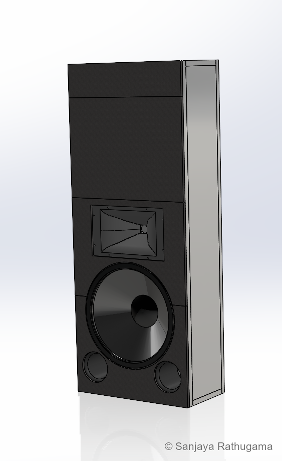
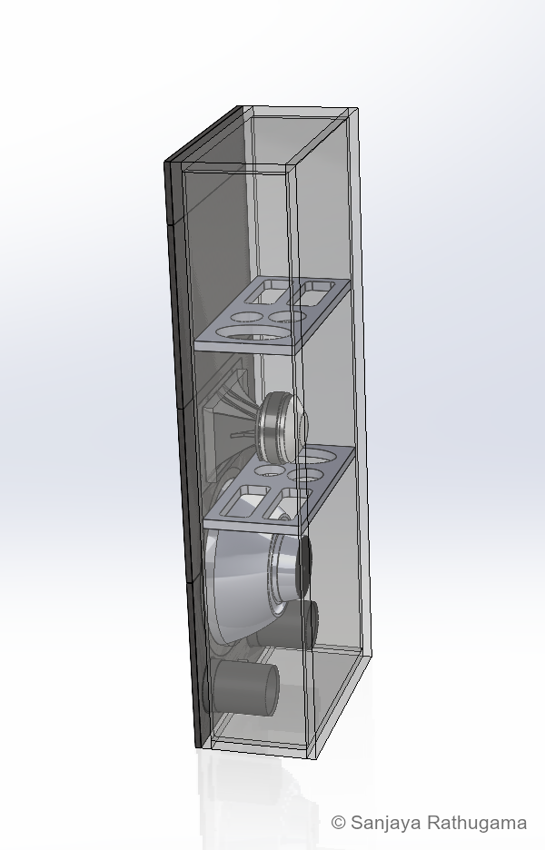
For the woofer I chose the SB Audience NERO-12MWN400D, paired with a ROSSO-44CD-PK compression driver. The NERO was probably overkill for this room, but home theatre does have a habit of encouraging that.
There was a practical reason behind it. Moving air depends on cone area and available excursion. Using the driver parameters in my enclosure model, the NERO offered roughly 2.4 times the cone area and 2.7 times the swept volume entered for the earlier BIANCO-8MW125 model. Those figures describe displacement capability, rather than a direct loudness multiplier. A larger cone can move the same volume of air with less travel, all else being equal.
The tradeoff was integration. The larger woofer needed a wider baffle and more enclosure space, and its upper-frequency radiation had to hand over sensibly to the horn.
The ROSSO-44CD-PK uses a PEEK diaphragm, a 44.3 mm voice coil and a ferrite motor, with a 25.4 mm exit to the horn. The exit size sets the horn connection; the much larger voice coil sits inside the compression driver. Its specified sensitivity made level matching with the woofer an important part of the crossover work.
| Part of the design | Configuration or target |
|---|---|
| Layout | Three matching vertical two-way LCR speakers |
| Cabinet shell | 1000 × 400 × 198 mm, height × width × depth |
| Woofer | SB Audience NERO-12MWN400D |
| Compression driver | SB Audience ROSSO-44CD-PK |
| Compression-driver construction | PEEK diaphragm, 44.3 mm voice coil, ferrite motor, 25.4 mm exit |
| Custom horn | Nominal 90° horizontal × 50° vertical target |
| Net enclosure model | 52.5 litres, tuned to 58 Hz |
| Ports | Two 80 mm internal-diameter ducts, approximately 112 mm long in the model |
| Driver crossover | Custom passive network developed in VituixCAD |
| Subwoofer handover | 80 Hz in the AVR |
The rectangular cavity in the CAD model is 968 × 368 × 164 mm, giving about 58.4 litres before subtracting the contents. Drivers, horn, braces and ports take up some of that space. The 52.5-litre figure is the net air-volume target used in WinISD, rather than the volume obtained by multiplying the cabinet's outside dimensions.
Choosing the bass alignment
WinISD let me investigate the bass alignment before committing to the cabinet. Volume, tuning and port dimensions were connected decisions: change one, then look at response, excursion and airflow together.
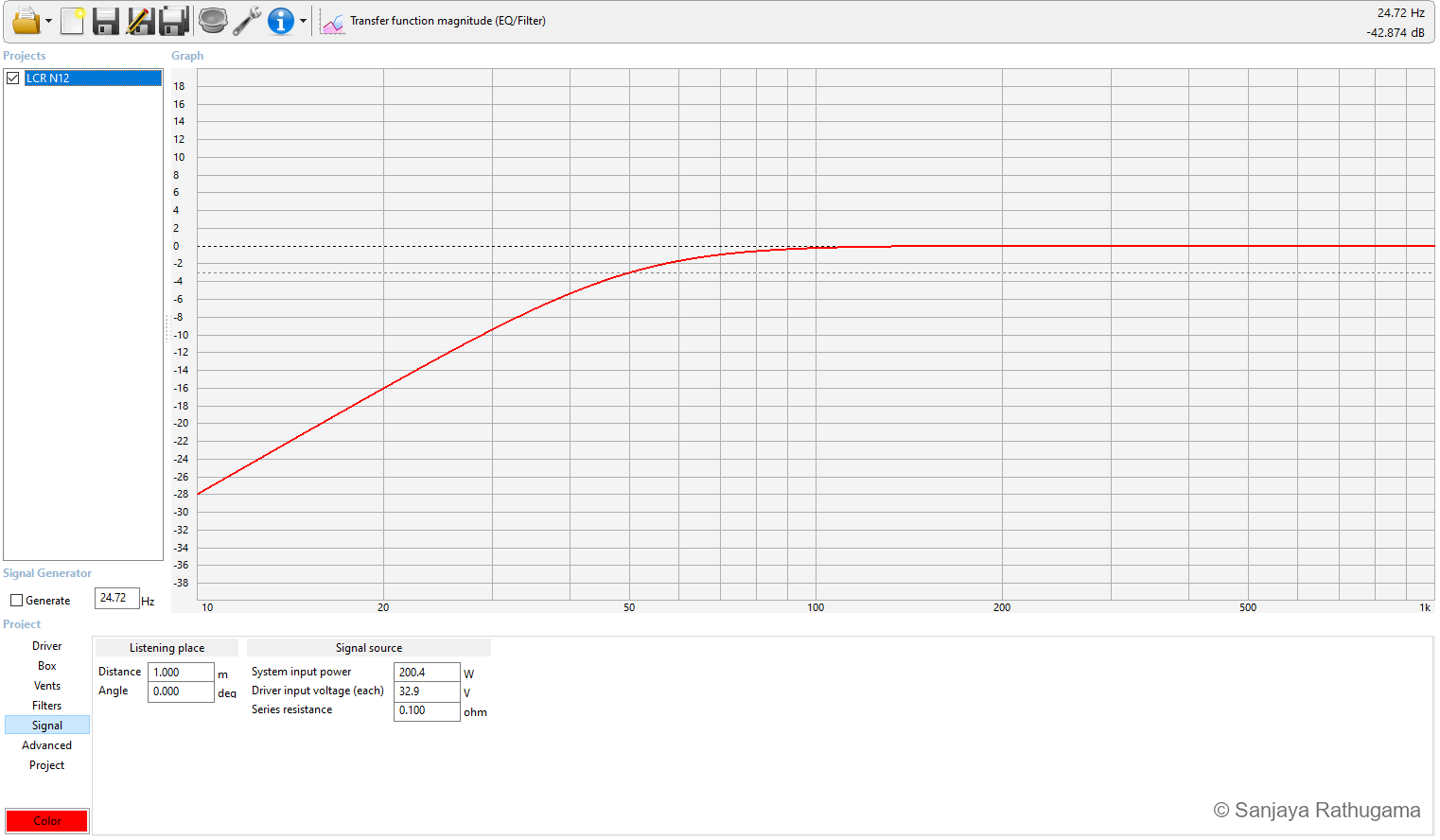
I modelled a 52.5-litre enclosure tuned to 58 Hz, with a 200.4 W input setting. WinISD's signal panel shows 32.9 V. Those are modelling conditions, rather than a rating for the complete passive speaker.
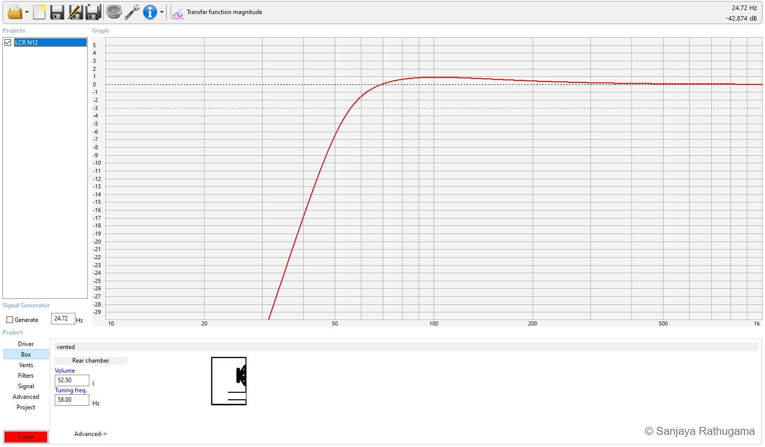
The model retained output below the planned bass handover, leaving room to integrate with the subwoofers. For the excursion and airflow checks, the study also included a second-order high-pass around 50 Hz. That filter condition matters when interpreting the results.
Two ports, and enough room for them to breathe
Two 80 mm ports provide about 100.5 cm² of total area, equivalent to one circular opening about 113 mm in diameter. Splitting that area into two ducts suited the front layout and the available enclosure depth.
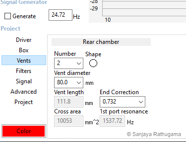
An earlier shallow-cabinet study used two 65 mm ports. Increasing their diameter to 80 mm added about 51 percent to the total area. At the same total volume flow, average air speed would fall by roughly a third. That was useful when trying to keep port noise out of demanding playback.
More area has a cost: retaining the same volume and tuning requires greater effective duct length. In a cabinet this shallow, a longer port quickly becomes a clearance problem. The entrance shapes and space around the inner ends matter as well as the number in the length box. Salvatti, Devantier and Button's port study (2002) examines how port geometry affects turbulence, compression and distortion.
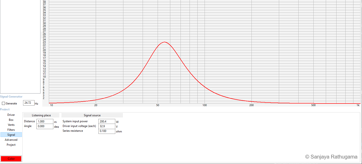
The 23 m/s peak belongs to that high-input design check. In the intended system, the AVR's 80 Hz bass-management crossover reduces the drive around 55 Hz, relieving the LCRs of much of the demand at the port-velocity peak. Its gradual roll-off leaves some output below the handover, so the full system has a different operating condition from the model shown here.
Predicted air speed alone does not establish audible chuffing. Port-end geometry, drive level and programme content all affect whether noise intrudes. In my system, I have not heard port chuffing, including during reference-level playback.
Check cone movement with the filter included
Near reflex tuning, port output becomes significant and cone excursion falls. Below that region, cone movement can rise while useful output falls. I needed to examine that behaviour alongside the frequency response.
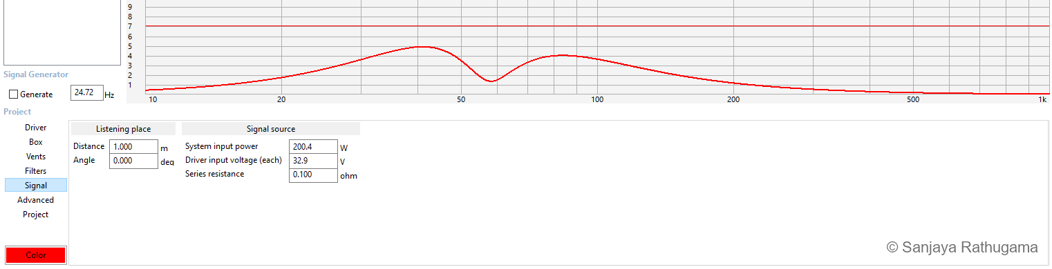
With the modelled input and filter conditions, predicted excursion stays below the entered Xmax limit. The dip near tuning shows the port taking a greater share of the output, with cone movement rising on either side.
These checks gave me a workable enclosure alignment to build and test. Predicting the complete speaker would also require its passive network: the inductors' winding resistance and the network's filtering change the drive delivered to the woofer. I continued with physical measurements as the cabinet and crossover came together.
A horn that would fit behind the baffle
The ROSSO compression driver needed an acoustic transition from its small exit to the room. Designing the horn in CAD let me work on the flare, mounting flange and clearances together. A deep horn plus the compression driver would consume the enclosure depth I was trying to save.
This is a custom compact horn/waveguide for the compression driver. The terms overlap: horn emphasises acoustic loading, while waveguide emphasises shaping the radiation pattern. I was working towards both in a shallow assembly.
The final horn targeted 90° horizontally and 50° vertically, widening the vertical target from the smaller prototype's 40°. The prototype article explains compression drivers and horn profiles; here the challenge was fitting the combination into the final LCR.
My geometry uses a rectangular mouth and a lofted, curved flare. The horizontal and vertical guide angles are 45° and 25°, corresponding to the intended included angles of 90° × 50°. A compact custom loft is a more accurate description than assigning it a textbook conical or exponential profile.
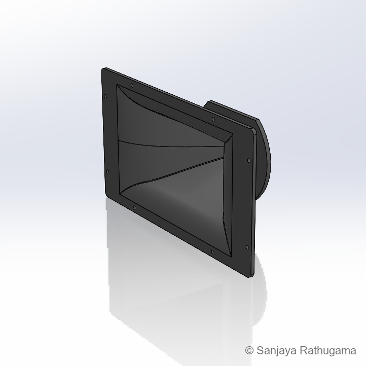
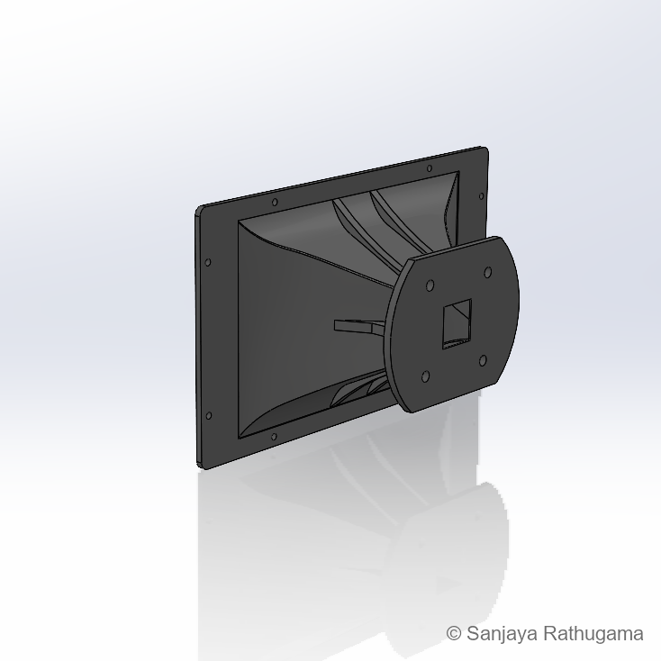
Those angles express the target. The mouth sketch is about 200 × 130 mm, while the wavelength at the approximately 1.68 kHz crossover target is about 204 mm. Near that region, diffraction, horn loading, driver behaviour and the woofer's contribution all matter. The finished speaker's dispersion cannot be obtained by doubling the CAD angles alone.
In the 3.6 m-wide theatre, the horizontal target was generous. It also made side-wall reflections part of the design problem. The technical notes explore the geometry in more detail.
From CAD to a cabinet on the bench
I started building the enclosures in mid-July 2024. Working with the actual panels brought the shallow design into focus: there was a large front face to assemble, but very little depth behind it for the drivers, horn, bracing and ports. Careful fitting mattered throughout the build.
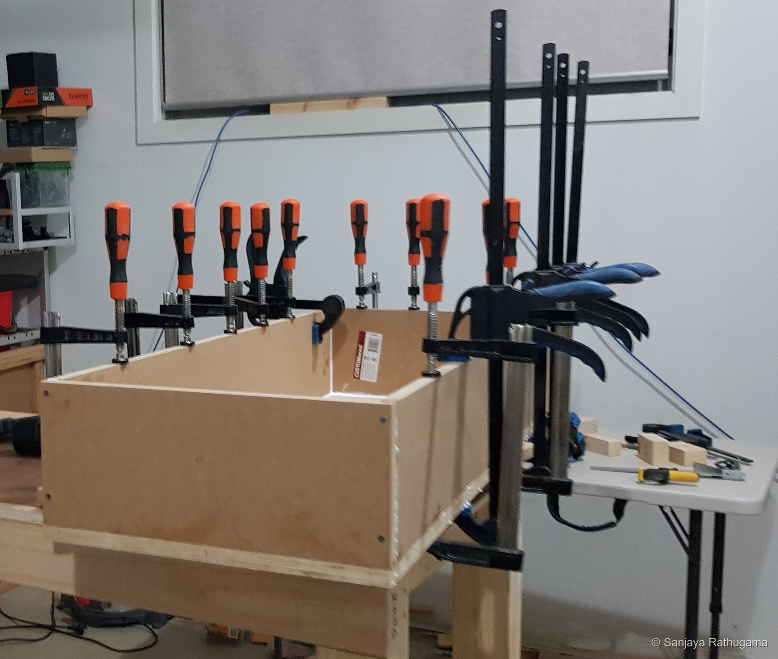
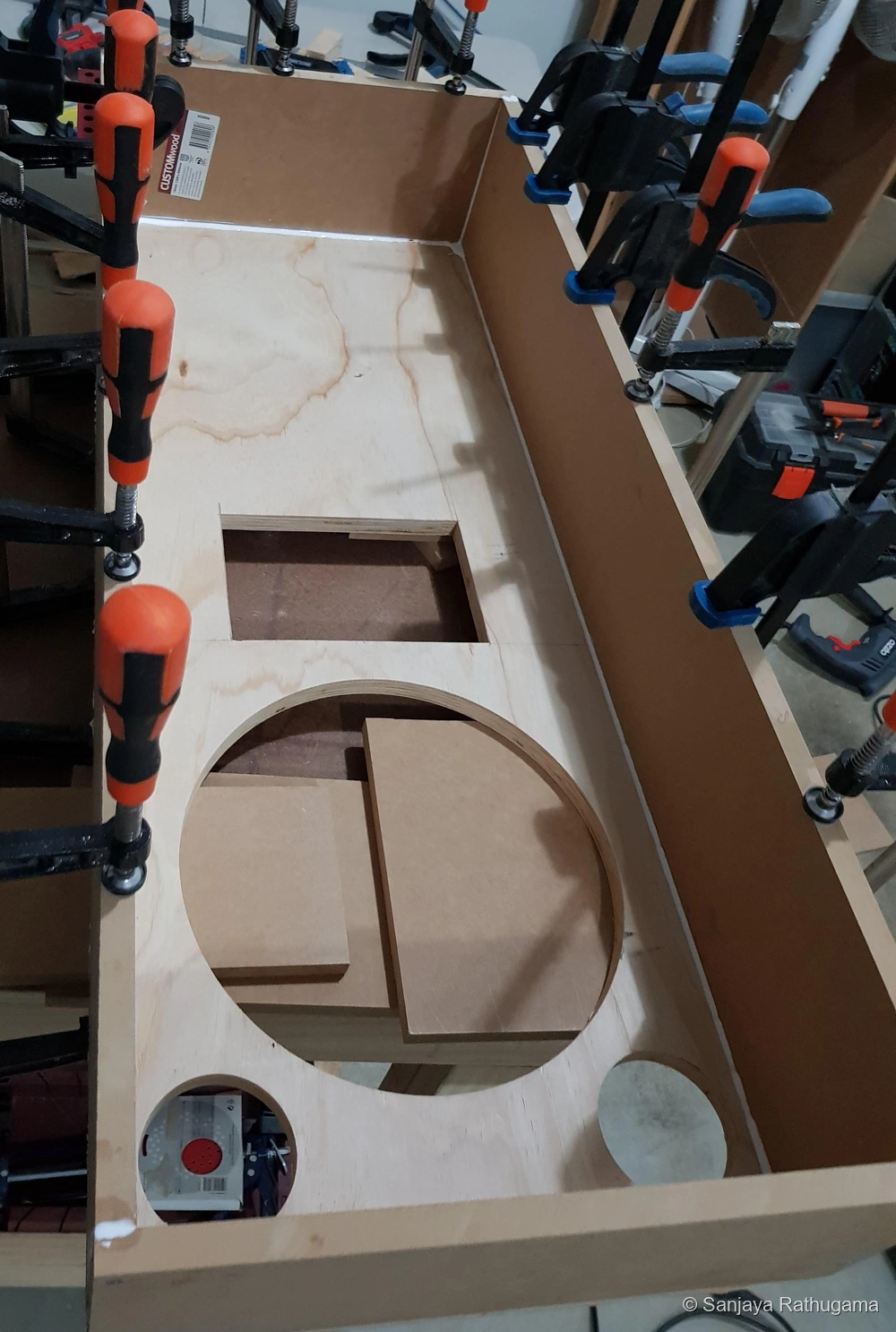
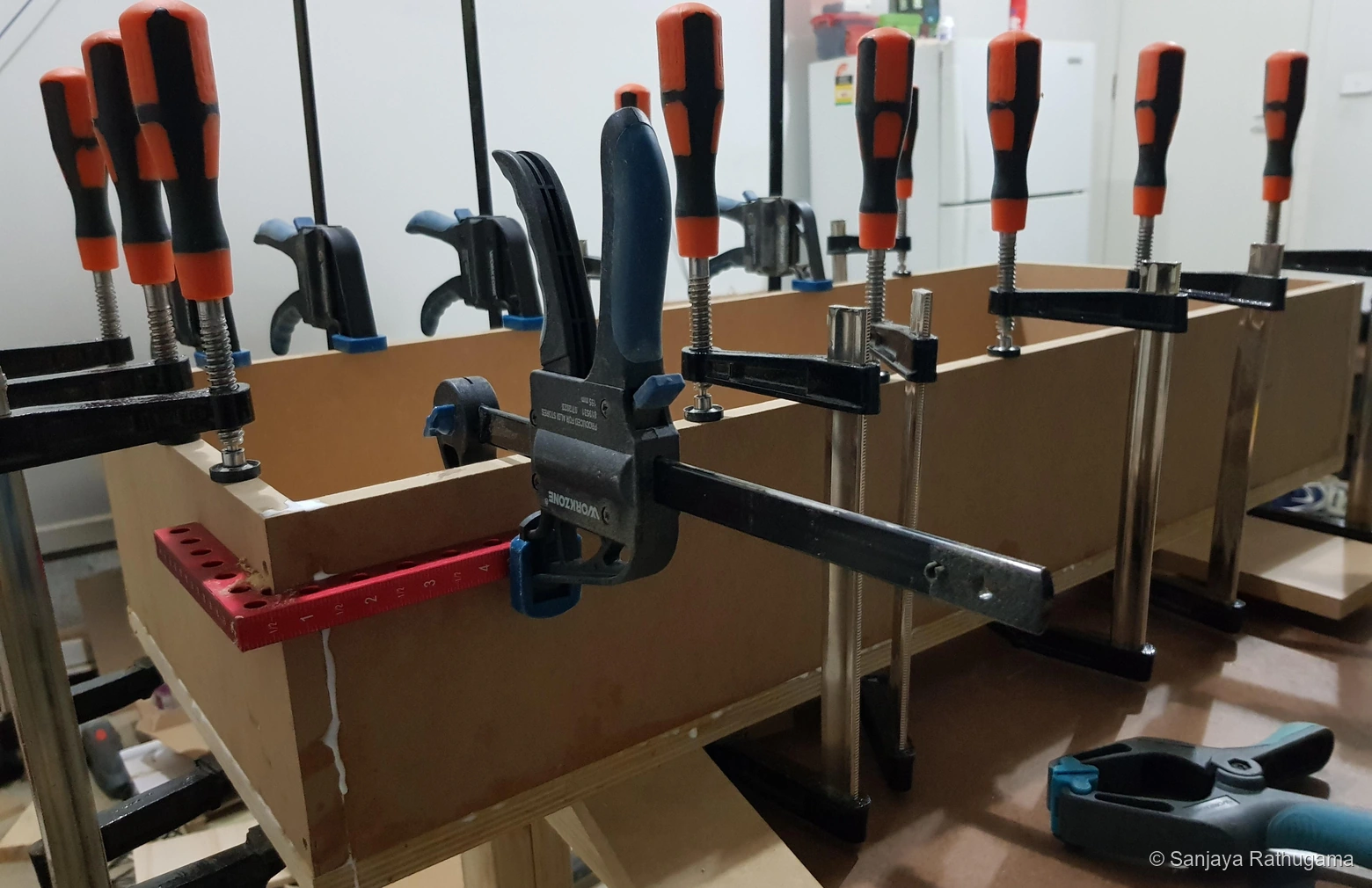
I used window-style bracing to tie the panels together and shorten unsupported spans. The openings left room for the drivers, wiring and airflow through the cabinet.
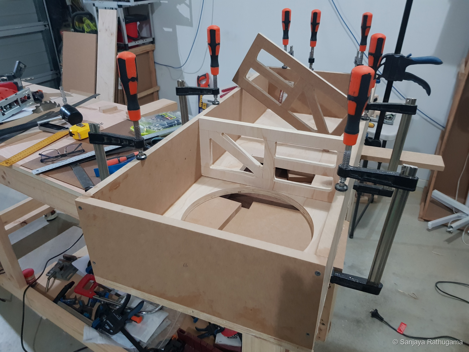
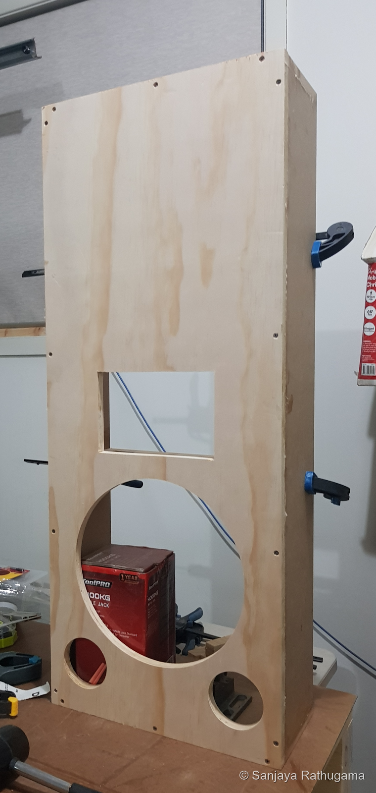
Getting the cut-outs in the right places was only part of the fit. Behind them I needed space for the baskets, fasteners, compression driver and port entrances. I also needed to be able to connect and service the assembly after those parts were installed.
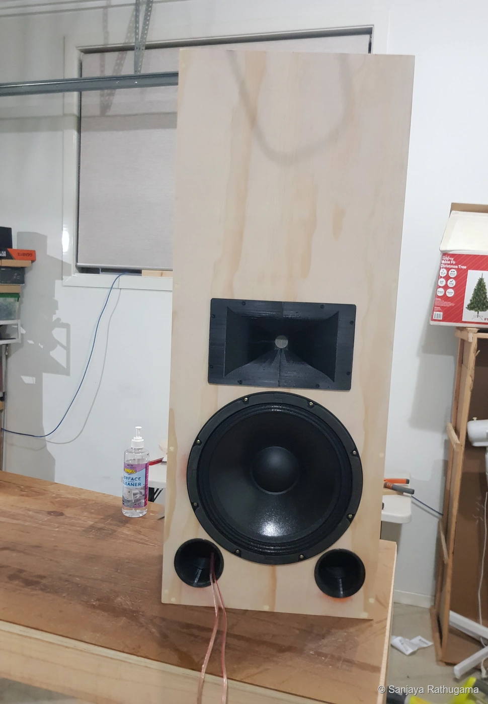
Horn development continued alongside the enclosure work. My home-built 3D printer made it practical to turn a geometry revision into something I could fit and test.
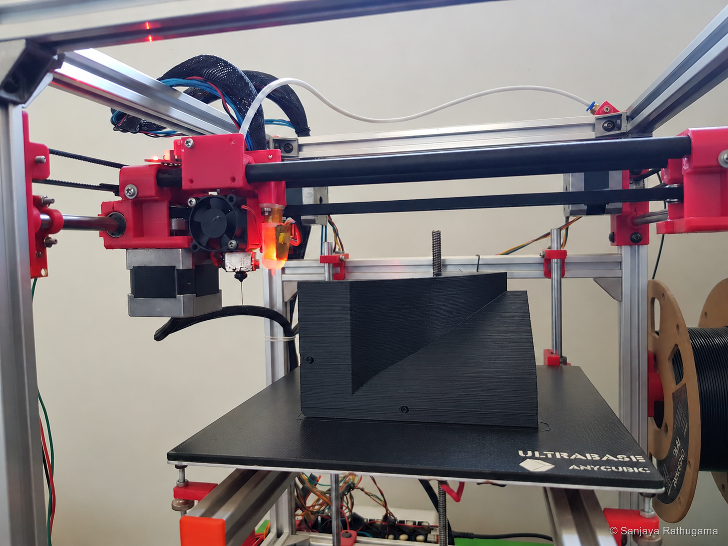
This was the same design, print, try and revise loop that had made the small prototype useful. A model could tell me whether parts intersected; the physical assembly told me how it actually went together.
Measure, change, measure again
Once the drivers were in a working enclosure and horn, I could start asking more useful questions about their behaviour together. I used a Behringer ECM8000 microphone, a Focusrite Scarlett 2i2 interface and REW. The design work and initial tests were done in my office, with its 2.4 m ceiling; the home-theatre room has a 2.72 m ceiling.
The crossover had to match their levels and manage the handover from the woofer to the horn, including how their outputs added around it. I measured individual drivers as well as combined configurations. That mattered whenever a change affected the handover region. A combined curve could show a change without explaining which driver had caused it.
During July and August I worked through driver levels, resistor and capacitor changes, lining placement, microphone height and temporary port closure. I kept notes against each reading so that a curve still meant something after the next change.
Matching the compression driver's level
The compression driver was sensitive enough that level matching needed attention. More high-frequency output did not automatically give a better-balanced speaker. In July I compared resistor values in its signal path while continuing to work on the woofer network.
The curves show the upper-range changes while much of the lower response stays similar. They helped connect a component change to its effect, rather than treating the crossover as a collection of independently chosen parts.
Lining and port experiments
The bracing restrained the panels; internal absorbent lining addressed the sound reflecting inside the cabinet. The back of the woofer radiates into that air space, where opposing surfaces can support standing waves. A shallow cabinet still has its longer height and width dimensions: simple empty-box estimates put the first axial modes around 177 Hz, 466 Hz and 1.05 kHz. The actual braces, contents and lining change that behaviour.
I used absorbent material inside the enclosure, then investigated its placement during measurement trials. The port entrances and air paths needed to stay clear, and I still needed access for fitting and servicing the components.
In August I compared changes to bottom damping, an external acoustic panel around the baffle and temporary port closure. The useful question was what each configuration changed. A modification did not become an improvement simply because I had spent time making it.
Compare the lining and temporary port-closure trials
Listening to a crossover before building it
Alongside the July measurements, I also used VituixCAD to build a bridge between a graph and a box of components. I exported individual driver filter responses as impulse-response files, then used convolution in Equalizer APO to audition the proposed crossover with separate output channels.
That made it practical to try a revision with the real drivers before committing it to passive hardware. Changing a value in a model is quick. Buying another inductor, rewiring a board and discovering that I preferred the previous version is rather less quick.
The digital trial remained part of the development process. A fixed filter represents the transfer function modelled for a particular load; the physical network still brings component tolerances, heating and changing driver behaviour. I needed to build and check it. These July listening trials preceded the October crossover revisions.
Developing the passive crossover
The NERO woofer and ROSSO compression driver differ in response, sensitivity, impedance and radiation. Their own behaviour is already present before the electrical filter does anything. Bringing measured responses into VituixCAD gave me a more useful starting point than nominal 8-ohm labels alone.
Choosing the handover involved a compromise. Let the woofer run too high and its narrowing radiation and upper-range behaviour become more relevant. Ask the compression driver to work too low and horn loading, excursion and distortion become concerns.
The later design targeted approximately 1.68 kHz, slightly below the manufacturer's 1.8 kHz recommendation in the datasheet available during development. That choice needs to be considered alongside acoustic roll-off, horn loading and playback level. The target frequency alone does not establish high-output protection.
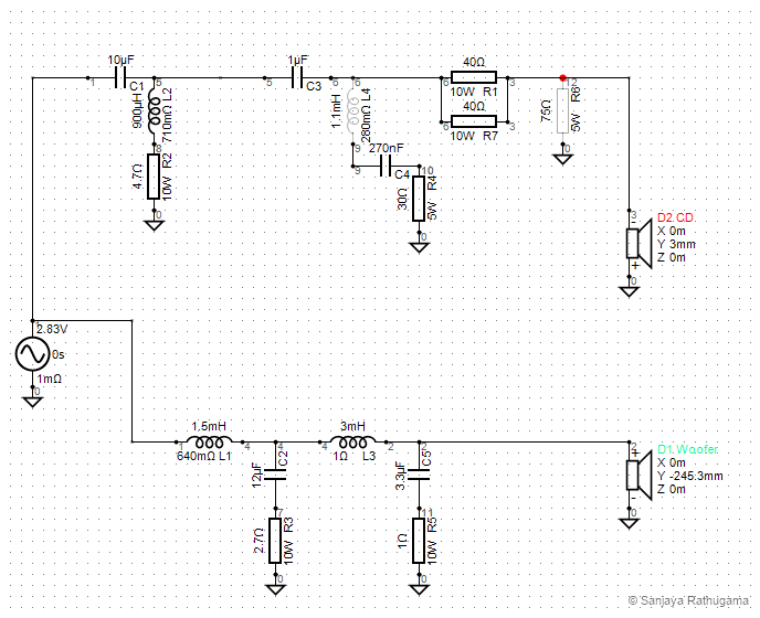
The woofer path includes series inductors and damped capacitor branches. The compression-driver path includes filtering and two 40-ohm resistors in parallel, giving 20 Ω of series resistance for attenuation. Those two resistors share the same pair of nodes, so they are not an L-pad.
The CD model is inverted relative to the woofer. That is a relative connection used in this design, rather than a rule that every two-way speaker should follow. L4 and R6 are open in the saved circuit; opening L4 also isolates the C4/R4 branch from the signal.
Open the complete VituixCAD workspace to see the calculated response, filter, phase and impedance panels alongside the circuit. Those plots depend on the imported driver data and its alignment. The polar and power-response panels do not establish measured dispersion without a complete off-axis data set.
Choosing the roll-off
The crossover frequency was only part of the decision. I also needed to control how quickly each driver stopped contributing beyond the handover. A nominal second-order filter approaches a 12 dB-per-octave roll-off in its stopband. That means approximately 12 dB more attenuation for each doubling of frequency above a low-pass transition, or each halving below a high-pass transition.
The final network developed into a tailored response rather than a simple textbook second-order pair. The woofer's two damped LC sections and the compression driver's capacitor, inductor and resistor network shape the slopes differently across frequency. Driver impedance also changes the electrical filtering, while the woofer's own response and the horn-loaded compression driver's behaviour contribute to the acoustic roll-off.
I therefore worked on the filtered driver responses and their overlap around the handover, using modelling, measurement and listening to guide each revision. A nominal filter-order label could not describe that whole result. The finished design should not be read as having a verified, constant 12 dB-per-octave acoustic slope on both drivers.
Bring the network into hardware
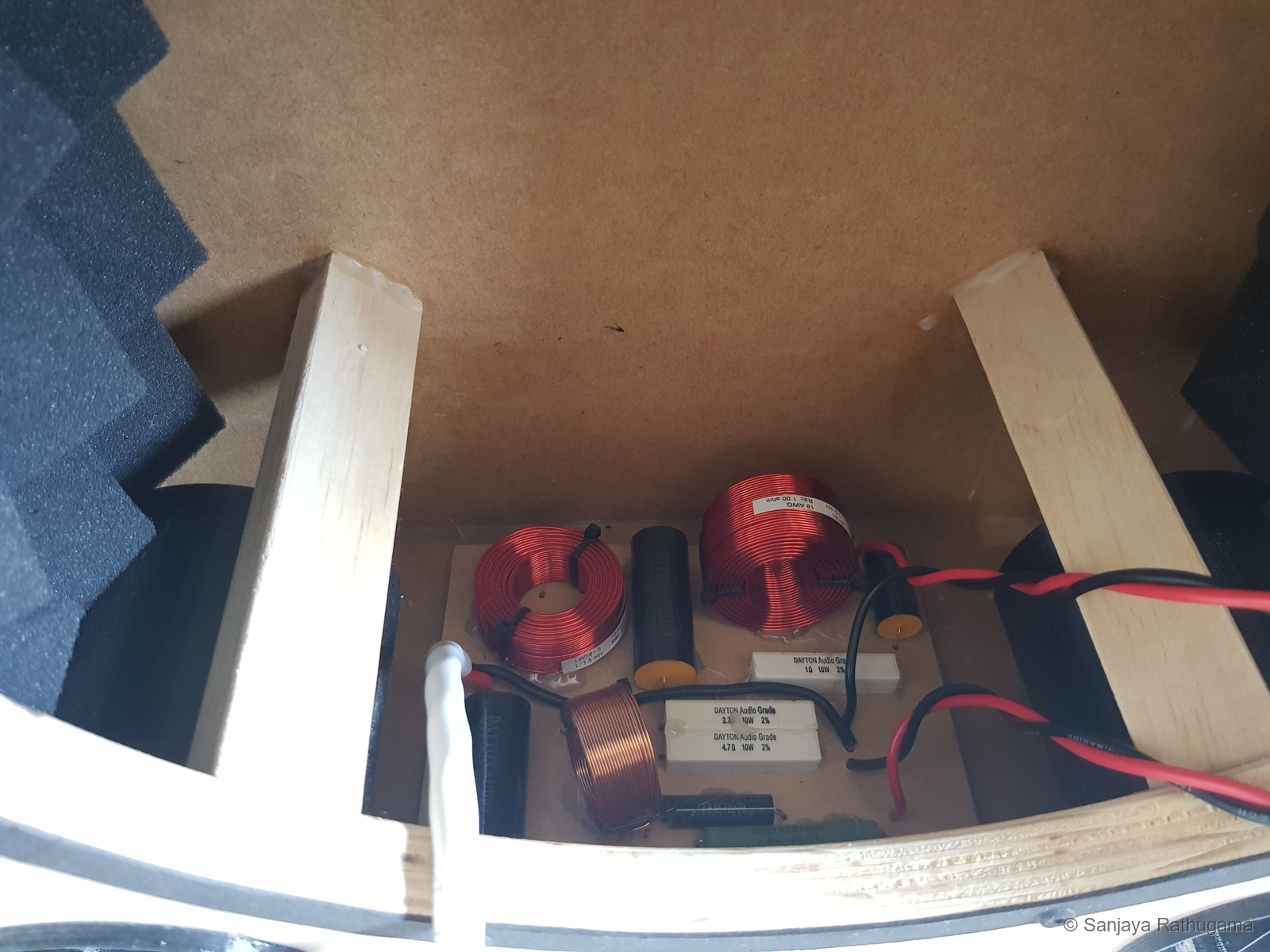
By October the physical test arrangement in my office still kept the crossover outside the cabinet. That left the components accessible while I continued checking the speaker. The room is approximately 3.7 m long, 3.09 m wide and 2.4 m high.
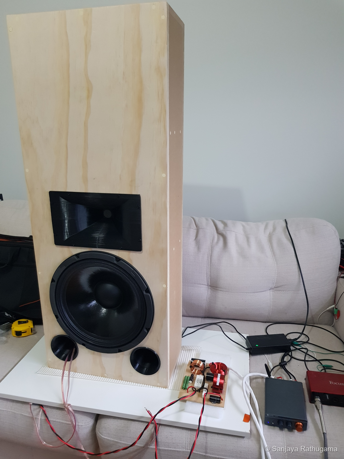
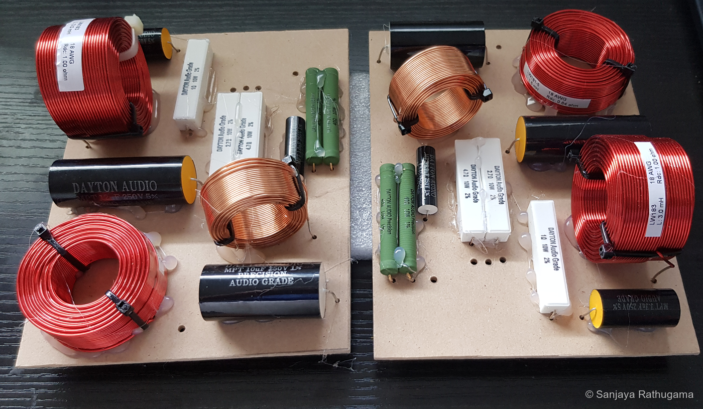
Building three matching networks brought component placement, secure mounting and repeatable assembly into the job too. The same circuit needed to become three consistently built boards.
Checking the assembled speakers in REW
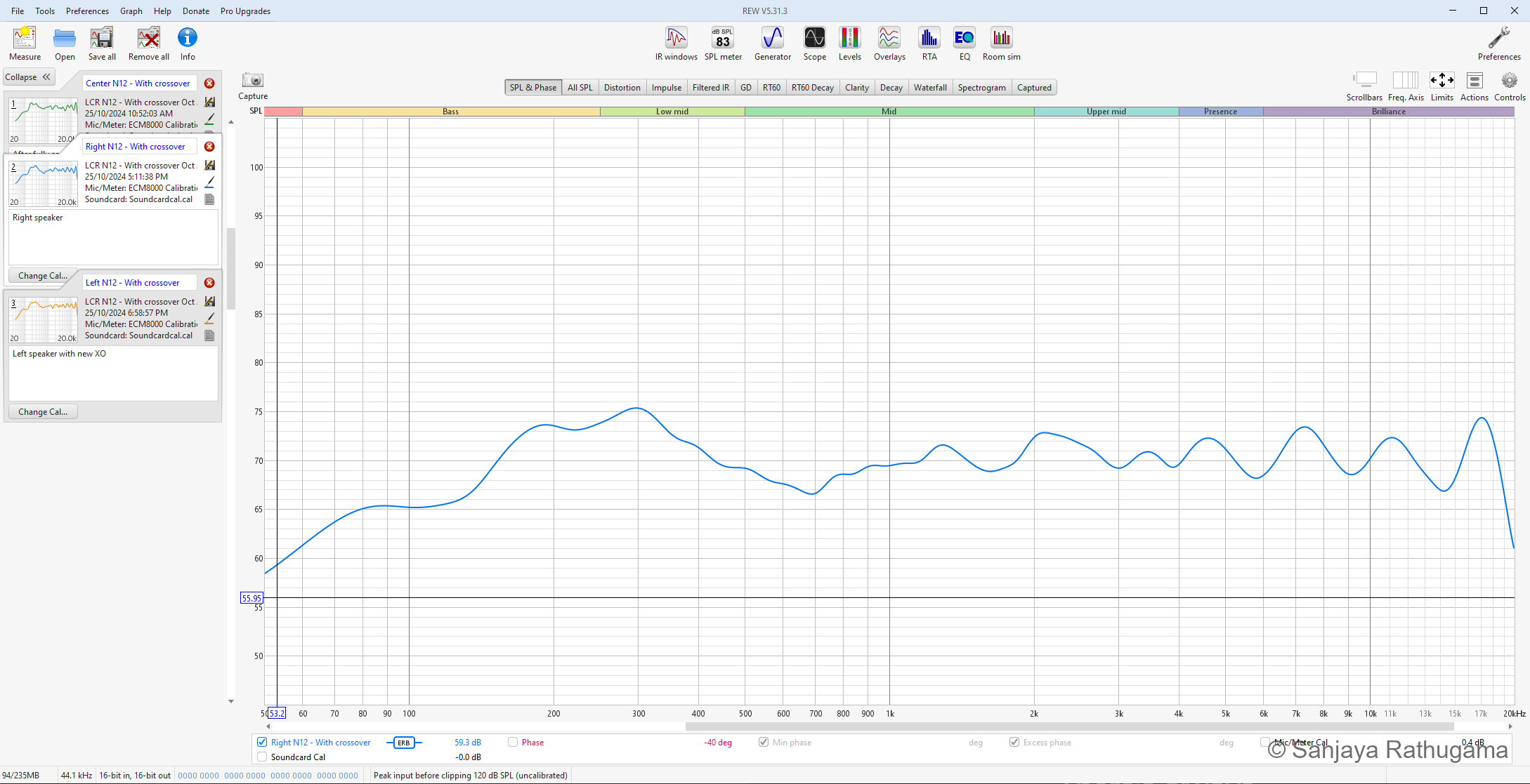
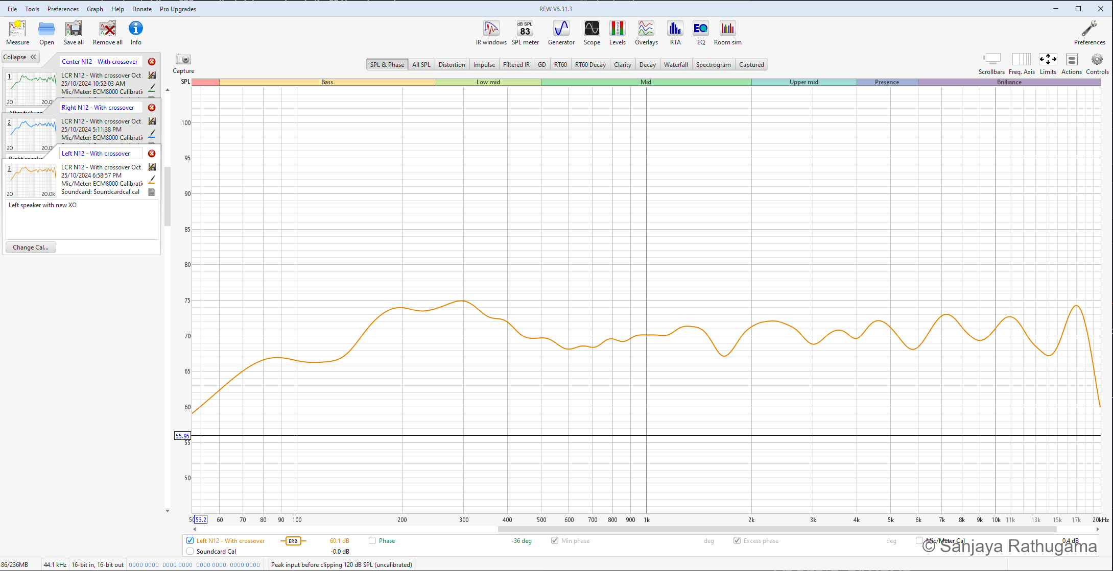
By 25 October, I had measurements of all three assembled speakers, including the left with its new crossover. Seeing the individual-driver experiments turn into complete speaker responses was a useful checkpoint before moving on to the AVR setup.
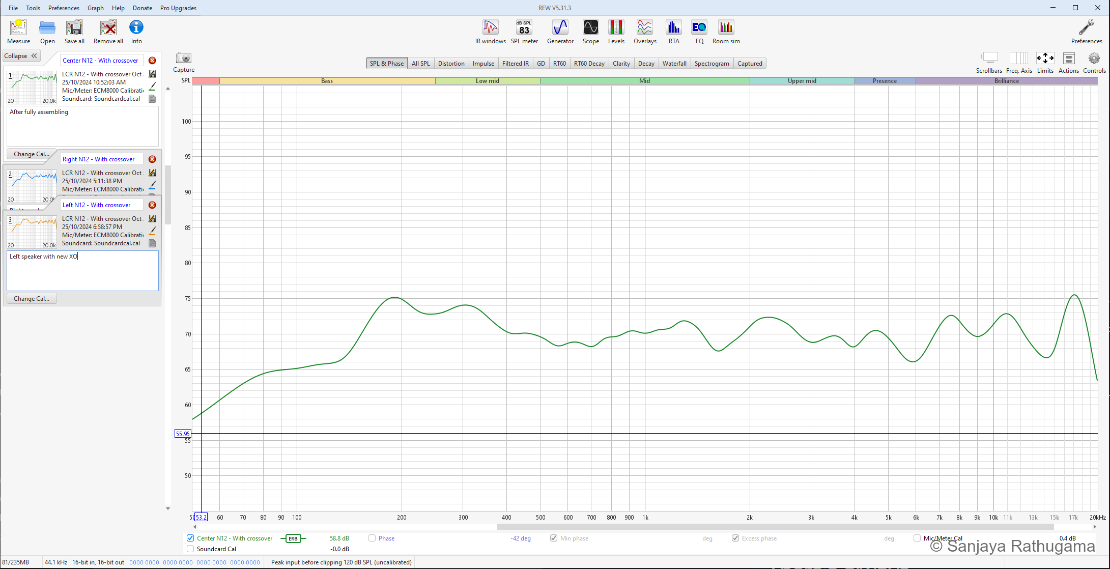
The broad shape was similar across the three speakers: an upper-bass rise, a modest depression around the crossover region and some remaining variation higher up. These tests were carried out in my untreated office room. The nearby wall and broad supporting surface could also influence the measured upper-bass balance. The curves alone do not separate those contributions from the speaker itself. I used the measurements to check the assembled result before the later theatre setup.
See the right and left speaker measurements
Measurement methods and limits
The July and August comparison graphs use the recorded 1/12-octave smoothing. Their impulse-response windows are around 20 ms, limiting deep-bass interpretation. The August set contains an ECM8000 microphone correction file; the earlier July entries do not. Frequency-response correction is separate from absolute SPL calibration, so the displayed levels do not establish sensitivity or maximum output.
The October screenshots use ERB smoothing to show overall tonal balance. Its heavier bass smoothing suppresses narrower features. These are development measurements made before Audyssey; the photographed office arrangement does not establish the exact microphone position or room setup for every sweep. They are not presented as a verified set of installed-theatre measurements. The screenshots show the historical measurements reopened in REW for this retrospective article.
The driver-response imports used in VituixCAD lack a documented common timing reference, and the imported impedance files contain magnitude without phase. The model helped guide revisions, but its calculated sum and load still depend on those inputs. A complete off-axis data set would be needed to assess the finished speaker's directivity and power response.
Three speakers in the front wall
I built the left and right speakers together. The centre followed a few weeks later, when I could make time for it. The design was a matching front stage, even though the three builds had to fit around the time I had available.
The final assembly brought the room constraint back into view. The cabinets sit within the developing front-wall structure around the window recess, preserving more of the room depth for seating.
The installed front stage is shown at the top of this article. All three speakers use the same vertical arrangement, woofer, compression driver and custom horn. The room treatment and finishing continued around them after the speakers were installed.
Once the speakers were in the theatre, the AVR's Audyssey setup was the next stage. REW had helped me refine the crossover and understand the uncorrected response. Audyssey's room correction then brought the system closer to the even balance I wanted in the listening area.
Dynamic EQ was part of how I used the finished system too. It works alongside room correction, adjusting tonal balance and surround presentation as playback level changes. That is a different task from the passive crossover, which integrates the drivers inside each speaker. Denon's AVR-X3600H owner's manual (2019, revised 2020) distinguishes MultEQ's room correction from Dynamic EQ's level-dependent compensation.
In use, the speakers have been very satisfying. The most rewarding part was hearing the project become part of watching films. The small prototype had given me somewhere to learn about the unfamiliar drivers and horns. The larger build required bringing that knowledge together with the enclosure, electronics, fabrication and the space I actually had.
What I would refine next
The driver-to-horn transition is one detail I would revisit. The driver has a 25.4 mm round exit, while the final CAD inlet is 25.4 mm square. Matching the width leaves extra area in the corners; a smoother transition could reduce reflections at that interface.
I have not identified an audible problem attributable to those corners. The existing response measurements cannot isolate them from the driver, flare and room. An otherwise identical comparison would be a useful next experiment.
A fuller set of time-referenced on- and off-axis measurements, together with complex impedance, would also make the next model more informative. The finished crossover's losses and the AVR's actual filtering belong in the complete system assessment. Those are ways to carry the experiment further while continuing to enjoy the speakers.
Technical notes and supporting plots
Enclosure alternatives and the WinISD model
| Saved NERO study | Net volume | Tuning | Ports | Length per port |
|---|---|---|---|---|
| Earlier larger-volume study | 65 L | 55 Hz | Two × 100 mm | 166 mm |
| Earlier shallow-cabinet study | 50 L | 58 Hz | Two × 65 mm | 70 mm |
| Later shallow-cabinet study | 52.5 L | 58 Hz | Two × 80 mm | 112 mm |
These were different enclosure studies. Their input and filter conditions also differ, so output and excursion comparisons need those conditions checked first.
The enclosure study includes 0.1 Ω source resistance, while the final woofer inductors total 1.64 Ω of saved winding resistance. The simple enclosure model therefore does not include the complete passive network. Its driver thermal-power field is also unset; it should not be used to publish a verified maximum-power rating.
The port settings estimate a first duct resonance around 1.54 kHz. That lies near the crossover region, making internal absorption and midrange leakage worth checking. The estimate alone does not establish an audible resonance in the finished speaker.
What the nominal horn angles mean in this room
The home-theatre room is approximately 4 m long, 3.6 m wide and 2.72 m high. The following centre-channel example assumes a horn mouth 0.2 m from the front wall, a horizontal axis at 1.2 m height and a listening plane 3 m from the mouth. The height and positions are illustrative, rather than surveyed installation dimensions. The left and right channels need their own positions and aiming included.
For an included angle θ, geometric span at distance d is 2 × d × tan(θ / 2).
| Distance from mouth | 90° horizontal span | 40° vertical span | 50° vertical span |
|---|---|---|---|
| 1 m | 2.00 m | 0.73 m | 0.93 m |
| 2 m | 4.00 m | 1.46 m | 1.87 m |
| 3 m | 6.00 m | 2.18 m | 2.80 m |
For the centred example, the nominal horizontal edges meet the side walls after 1.8 m. The 6 m span at the 3 m listening plane is already wider than the room. Boundary reflections remain relevant, and sound continues outside the nominal edges.
The 50° envelope meets the floor after about 2.57 m and the ceiling after 3.26 m. The 40° envelope meets the floor after about 3.30 m and the ceiling after 4.18 m, beyond the rear wall in this layout. Real vertical response also depends on driver spacing, phase and the crossover.
First-arrival geometry
Using 343 m/s for sound speed, a direct 3 m path takes about 8.75 ms. The image-source method gives a first side-wall path of about 4.69 m, arriving at 13.66 ms, and a rear-wall path of about 4.60 m, arriving at 13.41 ms.
Reflection strength depends on the frequency-dependent source radiation and the surfaces. Full system prediction would need measured polars, speaker and seat locations, crossover behaviour and room properties.
Amplification and bass-management details
Emotiva's XPA Gen3 manual, revision 3.2 from April 2018, specifies 200 W per channel into 8 Ω with all seven channels driven and 300 W per channel into 8 Ω with two channels driven. It also specifies support for 4 Ω loads. Those test conditions do not establish an exact three-channel rating. The historical manual is listed on Emotiva's manuals page.
The amplifier's available output was headroom, rather than power continuously delivered to every component. Film soundtracks have changing levels and frequency content. Average programme demand and sustained tones place different thermal loads on a crossover; the physical component ratings still matter when assessing the operating limits.
The LFE channel is separate from bass redirected out of the LCR channels. Its low-pass setting serves a different purpose from the speaker crossover. Neither the amplifier's rating nor an AVR menu setting establishes measured reference-level capability at every seat.
Further reading
Background references published before the 2024 development work. The cabinet dimensions, model settings and measurement history come from my own design and test records.
- SB Audience, ROSSO-44CD-PK datasheet, revision 2, 10 February 2022: compression-driver dimensions, 60 W AES rating, 107 dB sensitivity on the H250 test horn and 1.8 kHz recommended crossover. Those test conditions do not establish the output of my custom horn. The NERO enclosure calculations use the driver parameters entered in my 2024 WinISD models.
- Alex Salvatti, Allan Devantier and Douglas J. Button, Maximizing Performance from Loudspeaker Ports, Journal of the Audio Engineering Society, volume 50, January/February 2002: port geometry, turbulence and compression.
- Kimmo Saunisto, REW measurements for crossover simulation with VituixCAD 2, guide dated 21 January 2023: microphone calibration, timing reference, impedance and measurement geometry. The author's page identifies this dated guide separately from later software manuals.
- Emotiva, XPA Gen3 User Manual, revision 3.2, April 2018: amplifier specifications and their test conditions.
- Denon, AVR-X3600H Owner's Manual, North American edition, document 3520 10688 00AD, 2019 edition with November 2020 revision: MultEQ and Dynamic EQ.